
Applies to: Player 5.4/5.5/5.6 for ArcGIS Pro
AreaVol provides a volumetric estimate using an analog of pools and/or prospects. In this article we consider how to use AreaVol and an explanation of some of the key settings.
Create an AreaVol Estimate
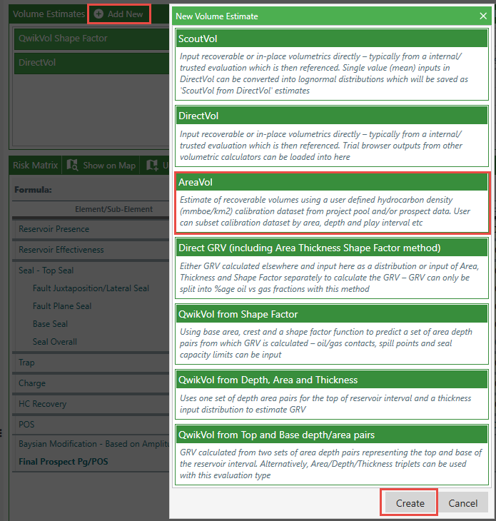
Open the Prospects dialog and navigate to the prospect target. Then from the Volume Estimates section select Add New > AreaVol > Create
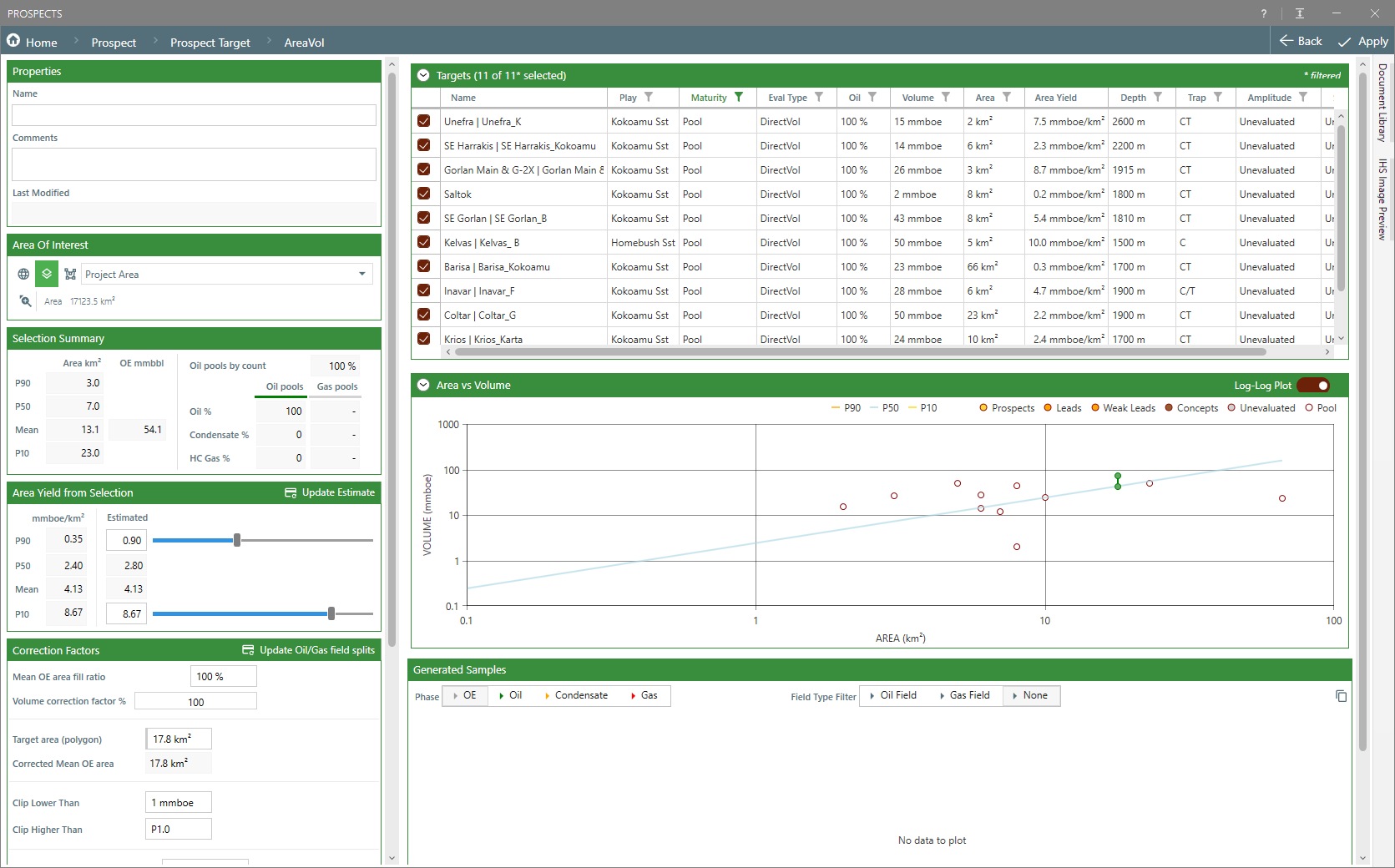
The AreaVol dialog will now appear showing a volumetric evaluation of an area
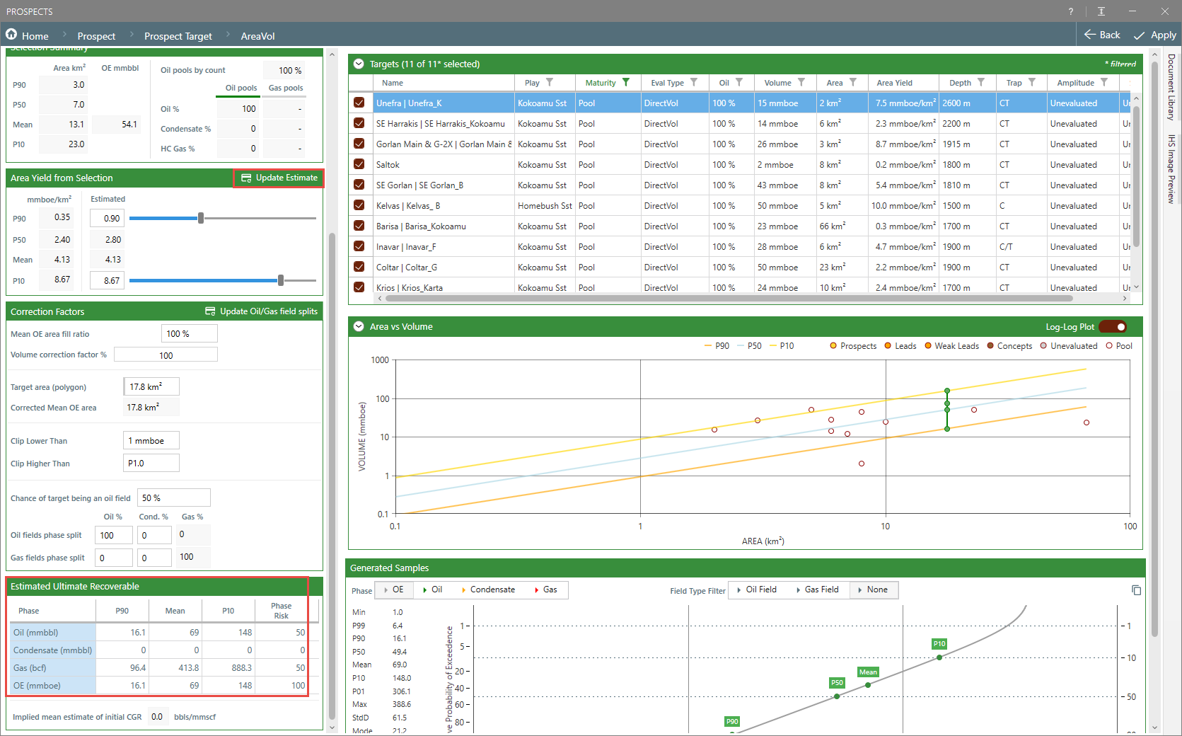
From the Area Yield from Selection select Update Estimate. This populates the graphs and volumes for the Estimated Ultimate Recoverable for the target.
Refining the Analog
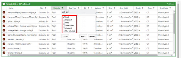
The Analog table shown above is also populated by area as defined by the Area of Interest options (Current Map Extent is selected in the example below)
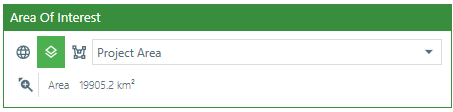
After applying any filters select Update Estimate from Area Yield from Selection
Analog Settings
The summary of the Analog table is shown in the Selection Summary. This is translated for the target in Area Yield from Selection. Volumes are per km squared. Pools are divided between oil and gas. We classify a field as an oil field if the volumes are >50% oil, gas otherwise. This figure is shown in the 'Oil pools by count'. In the example below we have 78.9% oil fields.
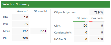
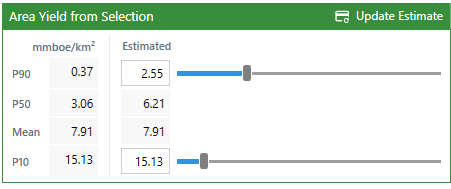
This value is then fitted to a distribution curve (so it will be close but may not be exactly the same) and shown in the Mean OE (mmboe)
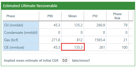
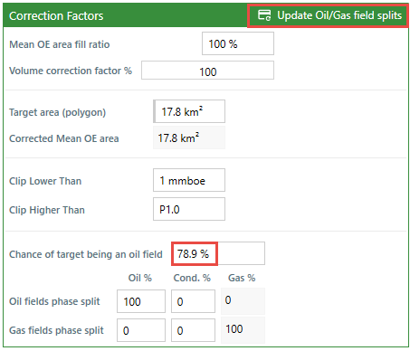
EUR OE (mmboe) are the volumes produced by the distribution curve. The volumes are disturbed between oil, condensate and gas depending on the phase split and phase risk. The Phase Risk is the possibility that there will be the phase present. OE (mmboe) will be the (phase values x phase risk) and then all phases for the column added together. In the example above the ‘chance of target being an oil field’ is 78.9%, so the chance of being a gas field is 21.1%, so we have volumes for gas.
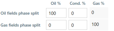
The phase split percentages is what percentage for a field having oil, condensate and gas volumes. The example above shows that any oil field will be 100% oil and any gas field will be 100% gas.
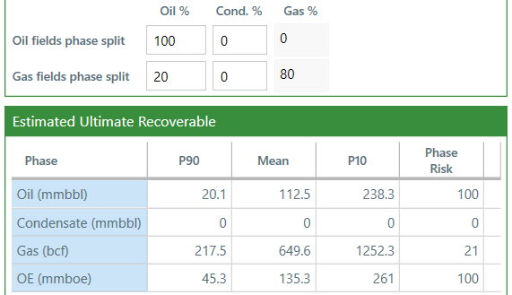
If we change the Gas fields phase split to 20% oil and 80% gas, counterintuitively the Oil Mean volume goes down from 135.2 to 112.5. This is because the Phase Risk has now changed from 79% to 100%. This is because every gas field now has 20% oil and we will therefore always have oil present. The OE Mean volume does not change when the phase split is changed as OE volumes is a total area yield calculation. So as the chance of oil has increased to take into account the gas volumes the oil volumes must decrease to honour the total OE volume.
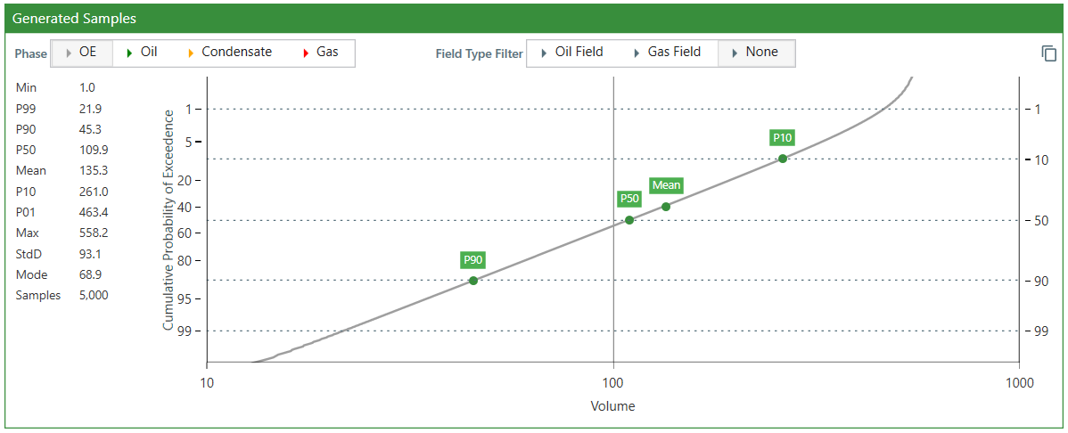
To save the AreaVol estimate select Apply and then Save